Simple Procedure to Design a Filter with Direct Coupled Resonators

Although computer market is full of all kind of sophisticated software able to “simulate” everything, the filter technology has not moved from 60-s at all. That time engineers designed filters of the same type without software and even without computers. Let assume the software can simulate any kind of magic structures. But where can we get that magic structures? By other word the software is not provided by a design procedure. However modern software allows using a big variety of new type of partial elements (not only irises, posts, etc.). Here below an approach to design a “direct-coupled” filter using a “simulator”.

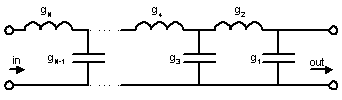
Low-pass filter prototype ladder network			Initially the low-pass prototype network elements values have to be found. They are normalized to roll-off frequency point (w) equal to unity and depends on the filter order and response type (Chebychev or maximally flat).
subroutine PreFilter(index,N,Lar,G) real G(30),a(30),b(30),Lar pi=3.141592653 eN=2*N if(index.eq.0)then do i=1,N e2=2*i-1 G(i)=2.*sin(pi*e2/eN) enddo endif if(index.eq.1)then xx=Lar/17.37 be=alog(cosh(xx)/sinh(xx))		v=sinh(be/eN) do i=1,N e2=2*i-1 a(i)=sin(pi*e2/eN) b(i)=v*v+(sin(i*pi/N))**2 enddo G(1)=2.*a(1)/v do i=2,N G(i)=4.*a(i-1)*a(i)/(b(i-1)*G(i-1)) enddo endif return end	There are simple expressions for g-values corresponding to Chebychev or Butterworth (maximally flat) responses in many microwave engineering books, for example, [1,2]. A fortran subroutine computing array of g-values from initial filter parameters is written in the left two sells of the table. The input parameters of the subroutine are index (0 for maximally flat or 1 for Chebychev), N (filter order), Lar (pass-band insertion loss ripple, dB).
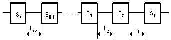
Network of s-parameters corresponding to filter structure The next step is to calculate reflection coefficients (S11) of each element of the filter at central frequency (b0)network required by the prototype. where Bi is equivalent susceptance of i-th element. Those values are obtained from the filter bandwidth (b1 - b2) and g-values using the expressions written on right.
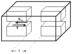
An filter partial element (brick). In case of filter based on double ridged waveguide the parameter may be the length of evanescent waveguide section.			After the reflection coefficients of network elements are found the network elements may be replaced by real elements providing the same reflection value at the filter central frequency. Such an element may be any kind of reactive discontinuity as iris, stub, evanescent mode section, post, etc. The reflection coefficient of that element has to be depended on a dimension parameter and vary in wide range if the parameter changes. For example, for an iris such a parameter may be width of the iris or its thickness. For inductive post it can be diameter of the post or distance to the waveguide wall. Actually there is no limitation what kind of discontinuities can be used to built a filter. It is just desirable to select all partial elements from the same family.
After those partial elements (filter bricks) are specified, the parameter values providing the prototype reflection values are to be found. To find those dimensions commercial software may be used. For many cases engineering formulas given in [1-4] for stubs, posts and irises may be used. The dimensions of each element (parameters) then may be found from a tabulated function of S11(b0,t) visually or using a numerical approach.
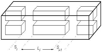
			After the dimension of each element is found, the distances between the elements can be also found. Distance between any two elements is associated with the phases of their reflection coefficients, ie where n is the resonance number. This length is usually called as cavity length despite for many structures, for example, evanescent mode ridged filter it may look like an iris or post.
subroutine Opti(Ns,N,fun,dx,x) real x(30),x0(30),Fx(30) external fun do istep=0,Ns F0=fun(N,x) print*, F0 Fn=0. do i=1,N call Variation(N,i,dx,x,x0) Fx(i)=(fun(N,x0)-F0)/dx Fn=Fn+(Fx(i))**2 enddo Fn=sqrt(Fn) do i=1,N x(i)=x(i)-Fx(i)/Fn*dx enddo enddo return end	subroutine Variation(N,i,dx,x0,x1) real x0(30),x1(30) do j=1,N if(j.ne.i)then x1(j)=x0(j) else x1(j)=x0(j)+dx endif enddo return end Ns is number of optimization steps, N is number of parameters, dx is increment, x is array of initial parameters and fun(N,x) is the function to be optimized		As the procedure is quite approximate, the obtained structure needs tuning elements or to be verified by an accurate software. Software based on mode-matching or integral equation numerical methods are better for this purpose than any kind of “mesh” software (see Software page). It is very likely that the filter response will need some corrections. The procedure can be repeated again and again until the filter roll-off and bandwidth are in right place. The reflection ripple (return loss) may also need adjustment.
			Commercial optimizers like OSA-90 may be used to improve and equalize the filter’s return loss. The most popular optimization techniques are MINIMAX and L2. These gradient methods may be easy realized in FORTRAN code, if a commercial optimizer is not available. A simple optimization subroutine is shown on left two cells of this table.